% fig16b.m - four-step gain, linear bandwidth
%
% -------------------------------------------------------------------------
% Copyright (c) 2005 by Sophocles J. Orfanidis
%
% Address: Sophocles J. Orfanidis
%          ECE Department, Rutgers University
%          94 Brett Road, Piscataway, NJ 08854-8058, USA
%
% Email:   orfanidi@ece.rutgers.edu
% Date:    June 15, 2005
%
% Reference: Sophocles J. Orfanidis, "High-Order Digital Parametric Equalizer
%            Design," J. Audio Eng. Soc., vol.53, pp. 1026-1046, November 2005.
%
% Web Page: http://www.ece.rutgers.edu/~orfanidi/hpeq
%
% tested with MATLAB R11.1 and R14
% -------------------------------------------------------------------------

clear all;

fs = 44100;
%fs = 96000;

N = 5; type=3;

L = floor(N/2);   % number of 2nd-order sections

G1 = 0; G2 = 18.0618;           % initial and final gains, G2 = 8 in absolute units
if type==0,
   gB = 3;                % Butterworth case
else
   gB = 0.01;             % Chebyshev and elliptic cases
end

G0 = 0; gs = 0.01;

N1 = 1000; N2 = 2000; N3 = 3000;

f0 = 400;                   % equalizer center frequency
Df1 = 20;  Df2 = 100;       % beginning and ending bandwidths

fsig = 400; wsig = 2*pi*fsig/fs;    % frequency of sinusoid

for n=1:N3+1,
  if n<=N1+1,
     Df(n) = Df1;
     G(n) = G1;
  elseif n<=N2+1,
     Df(n) = Df1 + (Df2-Df1)/(N2-N1) * (n-N1-1);
     G(n) = G1 + (G2-G1)/(N2-N1) * (n-N1-1);       % linear change in dB
  else
     Df(n) = Df2;
     G(n) = G2;
   end
  if G(n)<gB,
     GB(n) = G(n)/2;
  else
     GB(n) = G(n)-gB;
     if type==2, GB(n) = gB; end
  end
  if GB(n)<gs,
     Gs(n) = GB(n)/2;
  else
     Gs(n) = gs;
  end
end

M = 250;                                % G increases in four-steps (1000/250 = 4)
nq = M * floor((0:N3)/M) + 1;
G = G(nq); GB = GB(nq); Gs = Gs(nq);    % define stepped gains

w0 = 2*pi*f0/fs; Dw = 2*pi*Df/fs; c0 = cos(w0); s0 = sqrt(1-c0.^2);

U = zeros(L+1,4);      % frequency-shifted canonical internal states
V = zeros(L+1,4);      % frequency-shifted transposed internal states
W = zeros(L+1,4);      % frequency-shifted normalized lattice states
S = zeros(2,2,L+1);    % frequency-shifted state-space realization states
Z = zeros(L+1,8);      % frequency-shifted decoupled realization states

for n=1:N3+1,   % time-loop

  x(n) = sin(wsig*(n-1));

  switch type
     case {0,1,2}
        [Beq,Aeq,Bhat,Ahat] = hpeq(N, G0, G(n), GB(n), w0, Dw(n), type);
     case 3
        [Beq,Aeq,Bhat,Ahat] = hpeq(N, G0, G(n), GB(n), w0, Dw(n), 3, Gs(n));
  end

  [ycn(n),U] = df2filt(Bhat,Ahat,w0,x(n),U);        % canonical realization

  [ytr(n),V] = transpfilt(Bhat,Ahat,w0,x(n),V);     % transposed realization

  [gamma,d] = dir2latt(Bhat,Ahat);                  % get lattice coefficients

  [ynl(n),W] = nlattfilt(gamma,d,w0,x(n),W);        % normalized lattice realization

  [A,B,C,D] = dir2state(Bhat,Ahat);                 % get ABCD parameters

  [yst(n),S] = statefilt(A,B,C,D,w0,x(n),S);        % state-space realization

  [gamma,dec] = dir2decoup(Bhat,Ahat);              % decoupled realization

  [yde(n),Z] = decoupfilt(gamma,dec,w0,x(n),Z);

end   % time-loop

t = (0:N3); Gt = 10.^(G/20);

set(0,'DefaultAxesFontSize',15);

if 1

% ---------- canonical --------------------------
figure;

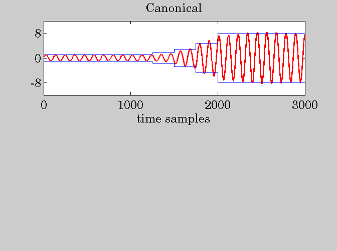
subplot(2,1,1);
plot(t,ycn,'-r');
hold on;
plot(t,Gt,'-b','LineWidth',0.5);
plot(t,-Gt,'-b','LineWidth',0.5);
hold off;
ylim([-12,12]); xlim([0,N3]);
ytick([-8,0,8]); xtick(0:1000:N3);
title('Canonical');
xlabel('time samples');
print -deps fig16b1.eps


% ---------- transposed --------------------------
figure;

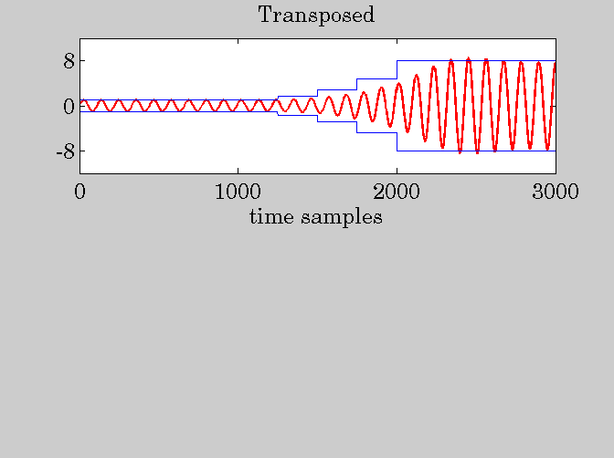
subplot(2,1,1);
plot(t,ytr,'-r');
hold on;
plot(t,Gt,'-b','LineWidth',0.5);
plot(t,-Gt,'-b','LineWidth',0.5);
hold off;
ylim([-12,12]); xlim([0,N3]);
ytick([-8,0,8]); xtick(0:1000:N3);
title('Transposed');
xlabel('time samples');
print -deps fig16b2.eps

% ---------- lattice -------------------------
figure;

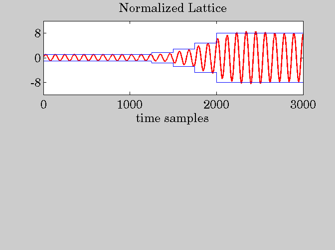
subplot(2,1,1);
plot(t,ynl,'-r');
hold on;
plot(t,Gt,'-b','LineWidth',0.5);
plot(t,-Gt,'-b','LineWidth',0.5);
hold off;
ylim([-12,12]); xlim([0,N3]);
ytick([-8,0,8]); xtick(0:1000:N3);
title('Normalized Lattice');
xlabel('time samples');
print -deps fig16b3.eps

% ---------- state-space ---------------------
figure;

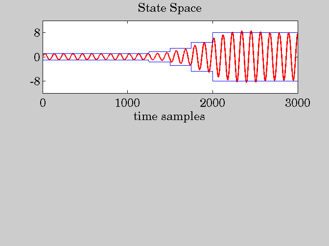
subplot(2,1,1);
plot(t,yst,'-r');
hold on;
plot(t,Gt,'-b','LineWidth',0.5);
plot(t,-Gt,'-b','LineWidth',0.5);
hold off;
ylim([-12,12]); xlim([0,N3]);
ytick([-8,0,8]); xtick(0:1000:N3);
title('State Space');
xlabel('time samples');
print -deps fig16b4.eps


% ---------- decoupled ---------------------
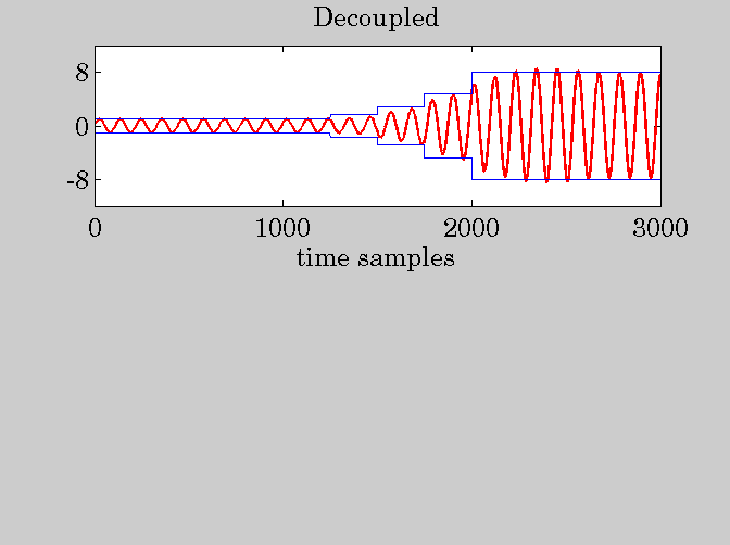
figure;

subplot(2,1,1);
plot(t,yde,'-r');
hold on;
plot(t,Gt,'-b','LineWidth',0.5);
plot(t,-Gt,'-b','LineWidth',0.5);
hold off;
ylim([-12,12]); xlim([0,N3]);
ytick([-8,0,8]); xtick(0:1000:N3);
title('Decoupled');
xlabel('time samples');
print -deps fig16b5.eps


end

Published with MATLAB® 7.0.4