% fig15.m - generates the graphs in Fig.15 of the paper:
%
% -------------------------------------------------------------------------
% Copyright (c) 2005 by Sophocles J. Orfanidis
%
% Address: Sophocles J. Orfanidis
%          ECE Department, Rutgers University
%          94 Brett Road, Piscataway, NJ 08854-8058, USA
%
% Email:   orfanidi@ece.rutgers.edu
% Date:    June 15, 2005
%
% Reference: Sophocles J. Orfanidis, "High-Order Digital Parametric Equalizer
%            Design," J. Audio Eng. Soc., vol.53, pp. 1026-1046, November 2005.
%
% Web Page: http://www.ece.rutgers.edu/~orfanidi/hpeq
%
% tested with MATLAB R11.1 and R14
% -------------------------------------------------------------------------

clear all;

fs = 44100;
%fs = 96000;


N = 5; type=3;

L = floor(N/2);

switch type
   case 0
      G0 = 0; G = 18; GB = 15; Gs = 0.01;
   case 1
      G0 = 0; G = 18; GB = 17.99;
   case 2
      G0 = 0; G = 18; GB = 0.01;
   case 3
      G0 = 0; G = 18; GB = 17.99; Gs = 0.01;
end

Na = 1000; Nb = 3000; Nc = 4000;

scale = 1;
fa = scale * 44.1; Dfa = scale * 22.05;
fb = scale * 441;  Dfb = scale * 220.5;
%fb=fa; Dfb=Dfa;
%fa=fb; Dfa=Dfb;

for n=1:Nc+1,
  if n<=Na+1,
     f0(n) = fa;
     Df(n) = Dfa;
  elseif n<=Nb+1,
     f0(n) = fa + (fb-fa)/(Nb-Na) * (n-Na-1);
     Df(n) = Dfa + (Dfb-Dfa)/(Nb-Na) * (n-Na-1);
  else
     f0(n) = fb;
     Df(n) = Dfb;
   end
end

w0 = 2*pi*f0/fs; Dw = 2*pi*Df/fs; c0 = cos(w0); s0 = sqrt(1-c0.^2);

U = zeros(L+1,4);   U1 = zeros(L+1,4);     % canonical internal states
V = zeros(L+1,4);   V1 = zeros(L+1,4);     % transposed internal states
W = zeros(L+1,4);   W1 = zeros(L+1,4);     % normalized lattice states
S = zeros(2,2,L+1); S1 = zeros(2,2,L+1);   % state-space realization states
Z = zeros(L+1,8);   Z1 = zeros(L+1,8);     % decoupled realization states

seed = 2005;  rand('state',seed);   % initialize random-number generator
x  = rand(1,Nc+1);           % random inout
x1 = 0.5 * ones(1,Nc+1);     % step input

for n=1:Nc+1,   % time-loop

  switch type
     case {0,1,2}
        [Beq,Aeq,Bhat,Ahat] = hpeq(N, G0, G, GB, w0(n), Dw(n), type);
     case 3
        [Beq,Aeq,Bhat,Ahat] = hpeq(N, G0, G, GB, w0(n), Dw(n), 3, Gs);
  end

  [ycn(n),U] = df2filt(Bhat,Ahat,w0(n),x(n),U);            % canonical realization - random input
  [ycn1(n),U1] = df2filt(Bhat,Ahat,w0(n),x1(n),U1);        % canonical realization - step input

  [ytr(n),V] = transpfilt(Bhat,Ahat,w0(n),x(n),V);         % transposed realization - random input
  [ytr1(n),V1] = transpfilt(Bhat,Ahat,w0(n),x1(n),V1);     % transposed realization - step input

  [gamma,d] = dir2latt(Bhat,Ahat);                         % get lattice coefficients

  [ynl(n),W] = nlattfilt(gamma,d,w0(n),x(n),W);            % normalized lattice realization - random input
  [ynl1(n),W1] = nlattfilt(gamma,d,w0(n),x1(n),W1);        % normalized lattice realization - step input

  [A,B,C,D] = dir2state(Bhat,Ahat);                        % get ABCD parameters

  [yst(n),S] = statefilt(A,B,C,D,w0(n),x(n),S);            % state-space realization - random input
  [yst1(n),S1] = statefilt(A,B,C,D,w0(n),x1(n),S1);        % state-space realization - step input

  [gamma,dec] = dir2decoup(Bhat,Ahat);                     % decoupled realization

  [yde(n),Z] = decoupfilt(gamma,dec,w0(n),x(n),Z);
  [yde1(n),Z1] = decoupfilt(gamma,dec,w0(n),x1(n),Z1);

end   % time-loop

t = (0:Nc);

set(0,'DefaultAxesFontSize',15);
%set(0,'DefaultAxesFontSize',10);


% ---------- canonical --------------------------
figure;

subplot(2,1,1);
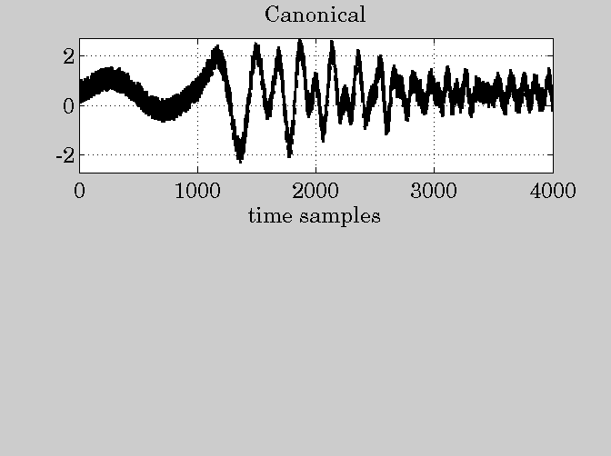
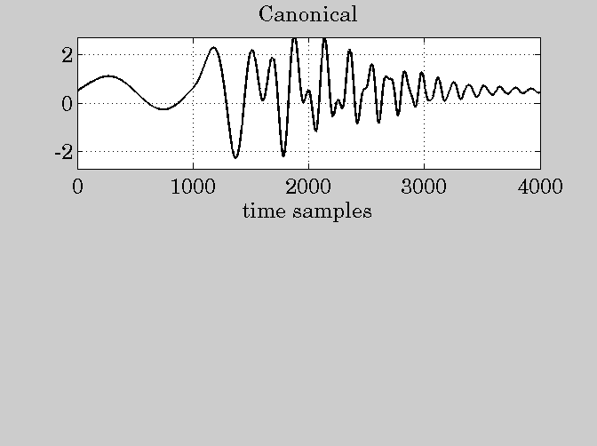
plot(t,ycn);
grid;
ylim([-2.7,2.7]);
title('Canonical');
xlabel('time samples');
print -deps fig15a.eps


% ---------- transposed --------------------------
figure;

subplot(2,1,1);
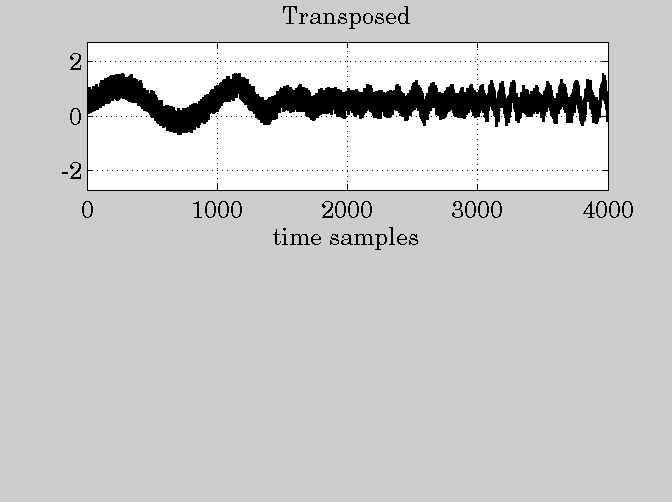
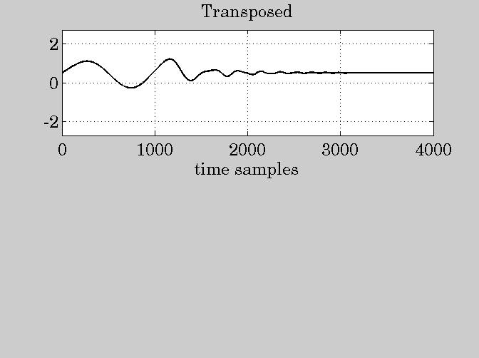
plot(t,ytr);
grid;
ylim([-2.7,2.7]);
title('Transposed');
xlabel('time samples');
print -deps fig15b.eps

% ---------- lattice -------------------------
figure;

subplot(2,1,1);
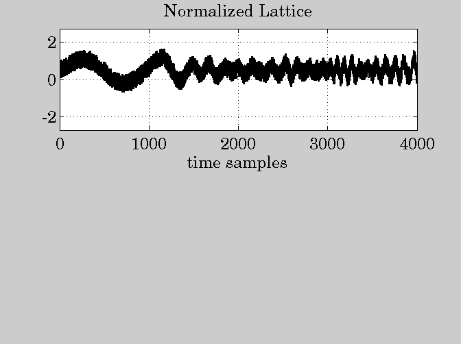
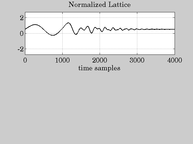
plot(t,ynl);
grid;
ylim([-2.7,2.7]);
title('Normalized Lattice');
xlabel('time samples');
print -deps fig15c.eps

% ---------- state-space ---------------------
figure;

subplot(2,1,1);
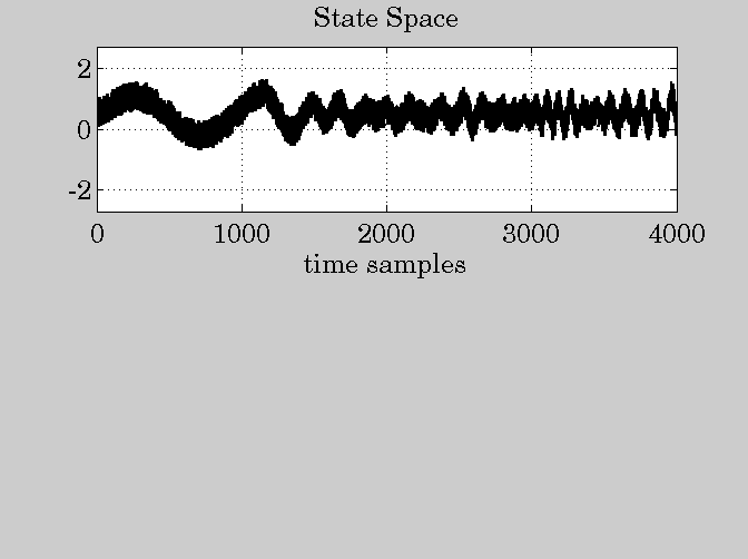
plot(t,yst);
grid;
ylim([-2.7,2.7]);
title('State Space');
xlabel('time samples');
print -deps fig15d.eps


% ---------- decoupled ---------------------
figure;

subplot(2,1,1);
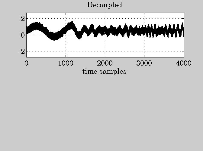
plot(t,yde);
grid;
ylim([-2.7,2.7]);
title('Decoupled');
xlabel('time samples');
print -deps fig15e.eps

% ------------------------ half-step responses ----------------

% ---------- canonical --------------------------
figure;

subplot(2,1,1);
plot(t,ycn1);
grid;
ylim([-2.7,2.7]);
title('Canonical');
xlabel('time samples');
print -deps fig15a1.eps


% ---------- transposed --------------------------
figure;

subplot(2,1,1);
plot(t,ytr1);
grid;
ylim([-2.7,2.7]);
title('Transposed');
xlabel('time samples');
print -deps fig15b1.eps

% ---------- lattice -------------------------
figure;

subplot(2,1,1);
plot(t,ynl1);
grid;
ylim([-2.7,2.7]);
title('Normalized Lattice');
xlabel('time samples');
print -deps fig15c1.eps

% ---------- state-space ---------------------
figure;

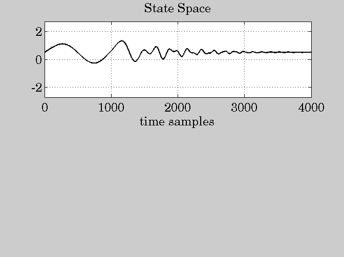
subplot(2,1,1);
plot(t,yst1);
grid;
ylim([-2.7,2.7]);
title('State Space');
xlabel('time samples');
print -deps fig15d1.eps


% ---------- decoupled ---------------------
figure;

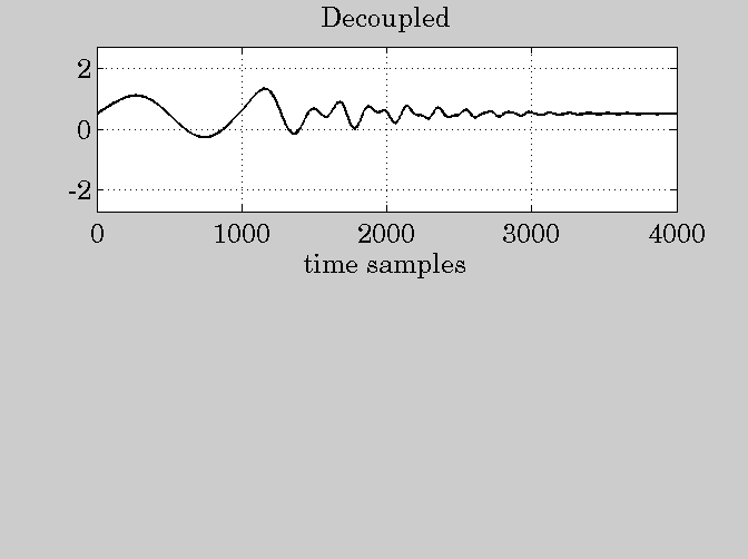
subplot(2,1,1);
plot(t,yde1);
grid;
ylim([-2.7,2.7]);
title('Decoupled');
xlabel('time samples');
print -deps fig15e1.eps

Published with MATLAB® 7.0.4